
Defining and quantifying compositional structure
What is compositionality? For those of us working in AI or cognitive neuroscience this question can appear easy at first, but becomes increasingly perplexing the more we think about it. We aren’t short on intuitions: we know that compositionality has something to do with reuse of parts, combinatorial expressive power, systematic generalization, and that natural language is a paradigmatic case, among other things. We seem to be able to glance at some data and say “yes, that is compositional!”, and we largely seem to agree on these judgments. But what is compositionality really, on a mathematical level, and can we quantify it?
Formalisms of intuitive concepts have proven incredibly useful in science, and for good reason. Humanity was long aware of things like gravity and drag, but it is only by understanding their deeper mathematical nature that we were able to build things like airplanes. We’re familiar with this phenomenon in AI as well. Since the early days of deep learning, people knew that building the structure of a modality and its symmetries into a model would be helpful, and were making some progress largely through intuition alone — for instance, designing convolutional architectures that are invariant to image translation1. However, it was only through the formalizations of Geometric Deep Learning2, which was built on the foundations of abstract algebra, topology, and group theory, that we were able to do this successfully in more general modalities such as graphs and manifolds. In contrast, when it comes to compositionality, we’re largely in the dark. We recognize its computational significance and its potential to address longstanding challenges like out-of-distribution generalization or continual learning, but we fumble around trying to make it emerge in our models without the proper theoretical tools needed to detect it, let alone build it in by design.
The purpose of this blog post is to introduce a formal definition of compositionality that provides unique value, beyond other notions that may be complementary. I don’t promise that it’s perfect — I have no experimental results and none of this has been vetted up to this point by peer review. Nevertheless, I feel like there’s enough here to warrant putting the ideas out in writing for the rest of the community to digest and criticize. As I hope you’ll find, the formal definition that I’m going to propose is both simple and wide-reaching, capturing disparate notions of compositionality within a single equation that applies to any form of data (a neural representation, a dataset, a piece of art or music, a physical object, etc.). I’ll also say quite a bit about what this definition of compositionality is useful for in AI, since it has deep implications for how we should build neural architectures and, even more importantly, how we should go about training them through the design of data curricula that maximize compositional structure. In all of these respects, it goes beyond a previous attempt of mine.
How to read this blog post
This blog post can broadly be divided into three sections. In the first part, I’ll introduce all of the ideas and key insights at a purely intuitive level, relying heavily on examples and analogies to make things as clear as possible on a first read. In the second part, I’ll make all of these ideas formally precise by expressing them through the mathematics of algorithmic information theory and compression, culminating in a single succinct equation that quantifies compositional structure. In the third and final section of the blog post, I’ll discuss some practical implications of these ideas for AI, touching on topics such as how to model hierarchical structure and construct data curricula from which knowledge can grow compositionally into the future, in a boundless and open-ended way. If you’re running out of steam by the end, I recommend you prioritize section 3’s entry on data curricula and open-endedness, as it is in my view the most consequential application of this definition of compositionality for the purposes of improving AI.
I’ve intentionally written the blog post in this fractured way to accommodate multiples styes of readers. For those who just want to get a sense of the ideas at a high level but tend to get bogged down in mathematical details as they come up, skip section 2 on a first read and only go back to it at the end if you still have the patience. For those who crave precision and formal rigour over more vague statements expressed in natural language, try to be lenient when reading section 1 and continue pushing through despite feelings of uncertainty, trusting that section 2 will resolve any ambiguity that was nagging at you. I should say at the outset that section 2 will inevitably be more tedious and might require more than one pass; it’s not that the math is complicated — there are no derivations, theorems, proofs, etc. — but rather that it builds off of branches of mathematics that are likely to be new to most readers (namely, algorithmic information theory). In the end, I promise that we’ll end up with a single succinct equation for compositional structure that is easy to interpret, even if the road that takes us there is a bit long and winding.
One more thing to flag is that I’ll occasionally make use of boxes for digressions, cumbersome clarifications, or another asides that risk breaking the flow of the overall text. These boxes are left purely for the sake of completeness, and readers should not feel pressured to delve into them, especially on a first read.
Section 1 — Compositionality as the emergence of novel shared structure
Paradigmatic examples of compositional data are easy to think of: a piece of music that recombines nested motifs and themes, an image dataset in which any given scene is made up of a combination of objects, a program that maximizes code reuse by defining a network of functions and classes, and of course natural language which can express an infinite set of ideas using a relatively small set of words and grammatical rules. Clearly, these examples have a lot in common, namely the notion of “parts” or “modules” which interact in complex cascades and at multiple scales to form the “whole” of the object.
This sort of multi-scale parts-based structure is what we’re going to try to quantify. To do so, I want to first drill down on the example of computer programs as a backdrop to our discussion that will extend more or less throughout the blog post. There are a few reasons for this. For one, programs are extremely general: any object we can think of can be described through a set of instructions (i.e., a program). Even more important, programs are paradigmatic cases of compositional objects that are familiar to all computer scientists. Once I’ve introduced all of the ideas in the context of computer programs, I’ll abstract them back out so that they apply to any object, be it a piece of music, a painting, an iid dataset, a nonstationary stream of data, a function, etc. — essentially, anything that can be thought of as information expressed in bits.
Programs and libraries
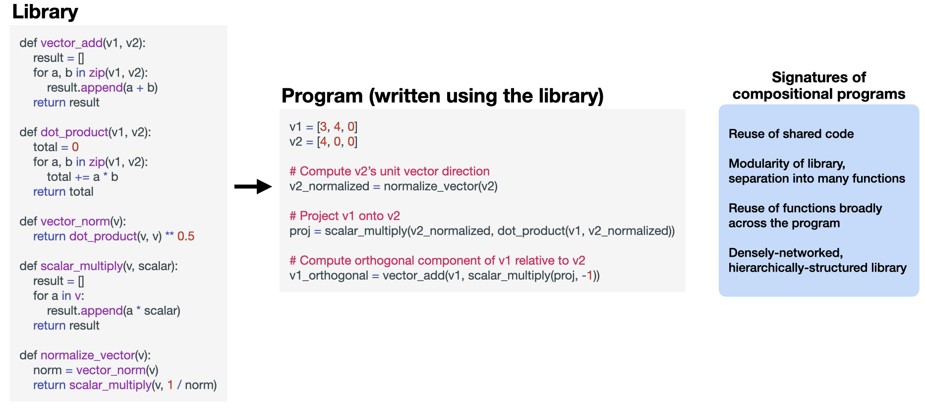
We consider some program compositional when it defines and reuses the same structures again and again in novel ways. Crucially, this is a property of the program’s library — the functions, classes, and data structures that it defines in order to optimize code reuse and modularity. By “library” here I want to stress that I do not mean an external package that one might import; I’m considering a self-contained program that makes no reference to external code, and the “library” refers to the reusable structures defined within the program itself — see the example in Figure 1. A compositional program’s library is rich, defining a number of functions and classes that serve as the “parts” which are recomposed. The structures in the library must also be broadly reused across the entire code base rather than only in local regions, otherwise we’re better off talking about multiple independent and non-compositional programs rather than a single compositional one. In addition, the libraries of compositional programs are themselves densely networked: functions and classes build hierarchically and laterally on top of existing ones.
I don’t think any of these high-level signatures of compositionality are particularly controversial. Formalizing these intuitions is more difficult, however: how do we move from qualitative and vague statements like the high-level signatures I outlined above to more quantitative ones that can be precisely expressed in mathematical expressions?
One of the key challenges is to specify which library we’re talking about, since any program can be implemented using an infinite number of possible libraries while remaining functionally identical. Is there any way to do this in a non-arbitrary way? For a given program that one might want to implement, is there a notion of the “correct” library one should write, or a library that is intrinsic to the program?
It turns out that there is, and it can be arrived at through the goal of compression. Think of what any good programmer would try to do: they would write the reusable code like functions and classes in a way that makes the total length of the program shortest. Other than for reasons of clarity, no programmer would insist on writing a function for some piece of code that is only going to be executed a single time in the program, because doing so wouldn’t help make the program more concise as a whole.
Growing and refactoring libraries
We now have a way of talking about a program’s intrinsic library as the one that leads to the best compression. To talk about compositionality, we want to quantify the degree to which this library is modular — whether it decomposes into multiple functions and classes that get reused in many places. We also want to quantify the degree to which this modularity is densely networked and hierarchical — whether some elements of the library are used to define other elements inside it, like some functions being recombined to define new ones.
If we can see the internals of the library and all of its components in detail, it might be possible to define some graph-theoretic metrics to quantify these things, but they risk being heuristic in nature and difficult to justify as truly general or theoretically-grounded. More problematically, while they may work for the specific case of quantifying compositional structure in programs, I’m primarily using programs as an intuition pump that we’ll later abstract out from. We’re looking for an approach that can just as easily be applied to arbitrary sorts of data like music, art, or datasets used for machine learning. In these other cases, the “library” that we’ll be talking about is less cleanly delineated into distinct modules and parts; clear boundaries might be fuzzy or non-existent, like the boundary between a solid or a liquid phase of matter, and we need our definition of compositionality to be robust here, too.
I’m therefore going to take another approach to defining the compositionality of a program that asks how the library grows or changes when we consider increasingly large segments of the program. Basically, if you imagine chunking up a program into some parts (i.e., non-overlapping segments of code), compositional structure exists when the best library for compressing those parts is different from the best library for compressing the whole. Why must this be true? If the library of the whole is different from the libraries of the parts (e.g., it has additional functions), it necessarily means that there were new shared pieces of code among those parts that could be placed in the library as new modules to improve compression. Conversely, if the library of the whole is identical to the libraries of the parts, then the whole program necessarily can’t be more or less compositional than its parts (compositionality is a property of the library, and the libraries are identical); it is just a longer program. It’s only when the library changes, or is refactored, that new compositional structure necessarily emerges. This definition of compositionality in the case of computer programs is summarized below:
Compositional program (in English)
A program is compositional with respect to some division into parts if the library that best compresses the whole differs from the libraries that best compress the parts.
I want to quickly clarify a few things before moving on. First, even when we consider joining parts to make a whole, we’re asking whether or not new compositional structure emerges; even if it does not, the parts themselves might already have compositional structure. This brings me to my second point: this definition of compositionality can be recursively applied to the parts themselves in order to investigate compositionality hierarchically at multiple scales. Finally, this recursive property raises the question of which hierarchical decomposition(s) we should consider, which I’ll have more to say about later in section 3.
Illustrative examples
For a very abstract definition such as this one, there’s no substitute for concrete examples that illustrate paradigmatic cases of both compositional and non-compositional structure. In some sense this is the entire goal of defining things in the first place — to include all positive cases while leaving out all negative ones using a simple expression — so lets put this one to the test. As before, I’ll make use of programs and libraries to build these concrete examples.
Brief notation
To avoid things getting to cumbersome, it’s time to introduce a tiny bit of notation. I’ll call a program $x$ and its best library (the one that best compresses it) $m_x$. I’ll denote the parts that we decomposed the program into with subscripts. We’ll just consider splitting the program into two parts for the moment, so that gives us $x_a$ and $x_b$ as well as their corresponding best libraries $m_{x_a}$ and $m_{x_b}$. We also said that we’re quantifying novel compositional structure as the degree to which the library of the whole changes from the libraries of the parts, which implies some sort of distance metric. We’ll call this distance $K(m_x \mid m_{x_a}, m_{x_b})$ for reasons that will become clearer in section 2.
Novel shared structure: compositional
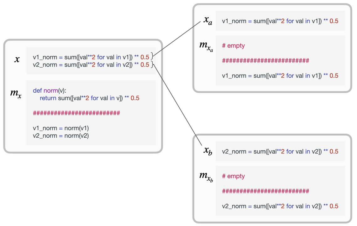
If $x_a$ and $x_b$ share some novel structure — for instance, pieces of code that could be turned into a function — then it makes sense to say that there’s additional compositional structure in $x$ that wasn’t already present in $x_a$ or $x_b$. This is exactly what is happening in the example of Figure 2, where in order to clearly show how a program is split into parts and which parts of the program share structure I have written them both with and without their libraries. In both $x_a$ and $x_b$, there was no sense in adding a norm() function to their respective libraries because there would have been no reuse; the overall programs would have been slightly longer if we had. Both the part libraries $m_{x_a}$ and $m_{x_b}$ are therefore empty. However, when we consider these parts together as a whole in $x$, suddenly it makes sense to write a norm() function to shorten the program because it will be used once.
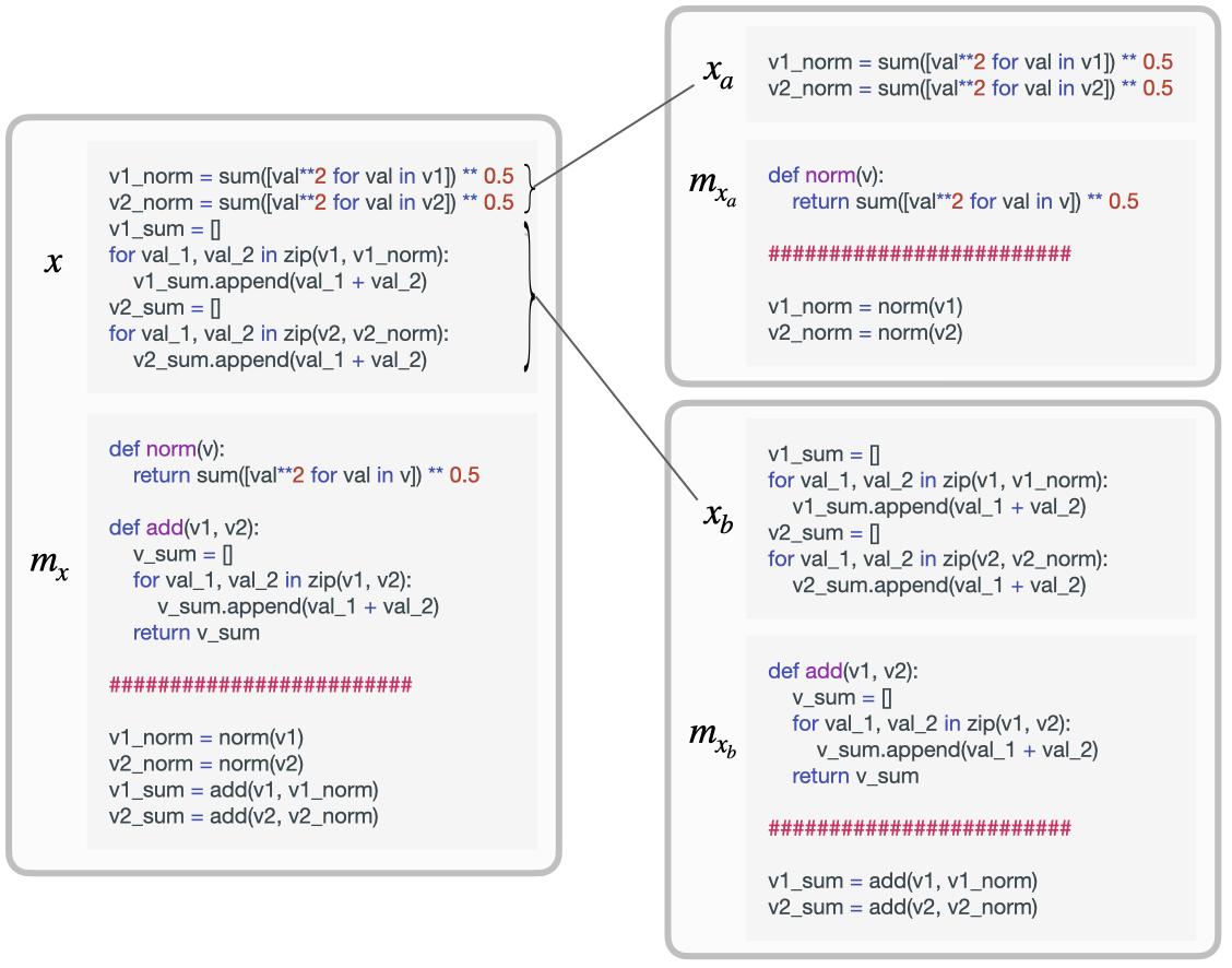
The definition I’ve proposed accounts for this: $m_{x_a}$ and $m_{x_b}$ in the example are both empty because there is no code reuse that would benefit from being wrapped in a function, but $m_x$ on the other hand is not empty, making $K(m_x \mid m_{x_a}, m_{x_b}) > 0$. This is the most minimal case of compositionality that we can construct — one “part” that is reused twice — and the definition correctly identifies it. Of course, the definition would also pick up on more interesting cases in which $m_{x_a}$ and $m_{x_b}$ might not be empty, and $x_a$ and $x_b$ share more interesting structure (e.g., multiple segments of code reuse that result in multiple new functions). In general, what happens in these sorts of cases is that the library of the whole $m_x$ grows with respect to the libraries of the parts $m_{x_a}$ and $m_{x_b}$, and this is always reflected in $K(m_x \mid m_{x_a}, m_{x_b}) > 0$.
It’s important to clarify once again what I mean by “novel shared structure” here. Clearly, the code that is shared between $x_a$ and $x_b$ was already present in each individually. However, when looking at those parts individually, the shared code does not show up in their libraries because it would not help us better compress them individually. It is only when we look at the combination $x = [x_a, x_b]$ that the shared code counts as compositional structure because it now helps us better compress the whole. The shared code itself is not what is novel, then, but rather the fact that this shared code now newly gets added to the library of the whole.
No shared structure: not compositional
A clear case that lacks compositional structure is when the best library we can build for $x$ just trivially combines those that were used for $x_a$ and $x_b$, such that $m_x = [m_{x_a}, m_{x_b}]$. This happens when $x_a$ and $x_b$ are unrelated to each other, such as in the example of Figure 3 where the two parts of a program serve entirely different functional purposes — in other words, they are algorithmically independent. Despite $m_x$ being larger and having more functions than either $m_{x_a}$ or $m_{x_b}$, it does not make sense to talk about $x$ as being more compositional than its parts $x_a$ and $x_b$ because those functions do not interact in any way. Instead, it makes more sense to talk about $x$ as two separate compositional parts that join together but do not compositionally interact with each other, almost like two separate subprograms that have nothing to do with each other.
My definition accounts for this case because the work involved in constructing $m_x$ from $m_{x_a}$ and $m_{x_b}$, which is quantified in $K(m_x \mid m_{x_a}, m_{x_b})$, is trivially small: the two libraries just need to be concatenated.
Fully shared structure: not compositional
Another case lacking compositional structure is when the library for $x$ is identical to the one used for either $x_a$ or $x_b$. Again, I need to emphasize here that we’re talking about additional compositional structure in the combination $x = [x_a, x_b]$; it is entirely possible that $x_a$ or $x_b$ themselves have rich libraries of reusable functions. But if the library for $x$ is identical to that of either $x_a$ or $x_b$, there is no reason to think of $x$ as being more compositional than its parts. This is the case when $x$ is nothing more than a longer program than $x_a$ or $x_b$ that is in fact reusing the same structures as them throughout.
Once again, my definition easily accounts for this case: $m_x$ is identical to one of $m_{x_a}$ or $m_{x_b}$, so it is trivially compressible from them.
Box: Compositional generalization
I want to give another quick example along these same lines, but this time in the realm of computer vision, since it has important connections to machine learning and generalization. While we’ve just spoken about programs up to this point, this brief digression will foreshadow how we’ll soon generalize the ideas up to this point to arbitrary kinds of data. Imagine that $x_a$ is a dataset of (concatenated) scene images and that $x_b$ is one additional image (nothing says the two objects have to be the same size). For the moment, we can think of the “libraries” in this case as “models” or collections of concepts (objects, possible relations between objects, etc.), although we’ll make this much more precise in section 2.
If $m_x = m_{x_a}$, it means that the new image $x_b$ consists entirely of known concepts, such that there is no additional structure it could provide. The new image $x_b$ contains the same objects, subparts, backgrounds, textures, and all other reusable structures that were already present in $m_{x_a}$. In this case, the best model of data $x_a$ is also the best explanation of $x = [x_a, x_b]$. This provides very general conditions under which we can meaningfully talk about compositional generalization and when it is even possible: a model can only compositionally generalize to new data, without undergoing additional learning, if that new data provides no additional compositional structure that would serve to change the model.
Building on top of existing structure: compositional
Lets now consider a more interesting example that will showcase the reach of the definition I’ve provided. A powerful benefit of compositionality is that it can allow us to describe some concepts as simple functions of others, whereas describing the concept from scratch might be pretty expensive. For instance, defining the concept of a “throne” without prior knowledge of concepts such as “chair” and “royalty” can be quite messy.
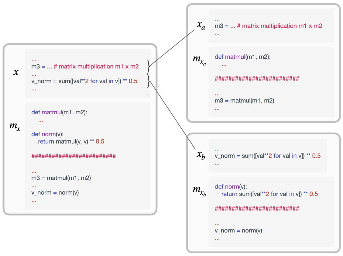
What does this look like for programs and libraries? Consider the example in Figure 4, where in the first part of a program $x_a$ we were doing a lot of linear algebra, and as such our library $m_{x_a}$ needed to define a function for matrix multiplication def matmul(a, b): .... Now, lets say that for the second part of our program $x_b$ we were doing some geometry that benefited from a vector norm function def norm(v): sqrt(sum([val ** 2 for val in v])). What will the optimal library $m_x$ look like when we consider $x_a$ and $x_b$ jointly? Crucially, the norm function will change in the new library because of novel shared structure between $x_a$ and $x_b$. In particular, $m_x$ will now define the function as def norm(a): sqrt(matmul(a, a)) because this is shorter once we already have code for implementing matrix multiplication. We have compositionality here because we get to re-express some concept (the norm of a vector) in terms of other concepts (matrix multiplication and square root). Crucially, in this case, it’s not that the library $m_x$ grew with respect to $[m_{x_a}, m_{x_b}]$, but that it was refactored from them because novel shared structure resulted in a better strategy for compression.
How does my definition account for this notion of compositionality? Effectively, we’ll have that $K(m_x \mid m_{x_a}, m_{x_a}) > 0$ because the implementation of the norm function in $m_x$ is a new component of the library — it was implemented differently in $m_{x_b}$, and has to be rewritten. Granted, in this example $K(m_x \mid m_{x_a}, m_{x_a})$ will be quite small since the new norm function is very easy to write given the matmul function in $m_{x_a}$, but the point I’m making is more general. Whenever novel structures or concepts can be succinctly described in terms of others, my definition correctly identifies this as a case of compositionality.
Generalization to any object: good libraries as Occam’s razor models
I hope that the above discussion of programs and libraries has been helpful for building intuition about compositionality, but ultimately we need to generalize outside of this particular case. For this, we’ll be replacing the notion of a program with that of any arbitrary data that can be expressed in bits. This encompasses things like music, images, iid datasets, non-stationary data streams, neural representations, functions, natural language utterances, computer programs — basically, anything that is scientifically interesting. The bigger question is: what should we replace the notion of the program’s library with? The analogous concept turns out to be a model of the data.
A model, like a program’s library, captures structure in the data: patterns of information that repeat in some shape or form, either in a quite literal sense (like a repeating subsequence of bits) or in more abstract ways (like a rule or template with adjustable parameters). Just like in a computer program, the patterns of information captured by a model can be interdependent and hierarchically-defined, like in a deep neural network where representations are built upon each other.
What all this means is that a model, like a program’s library, can compress the data in ways we’ll make more precise in section 2. A model can be thought of as a shorter explanation of a more complex object. If I give you a pattern of bits like 01001100011100001111... and ask you what’s going on, you’ll probably say something like “alternate groups of 0’s and 1’s and increase the group size by one each time” — that’s a model of the data (in this case a generative one) that can help us compress the string with far fewer bits because the model is simple and easy to encode. Even if the model isn’t perfect and has some degree of error (e.g., imagine corrupting the above string with a bit of noise), it can still help with compression because encoding the model along with a few error-correcting bits can be easier than encoding the entire string verbatim.
Box: Models of individual objects rather than datasets
I want to quickly head off a potential confusion for the machine learning audience. We’re accustomed to modeling datasets (often iid ones), and so the idea of modeling an individual object or a nonstationary stream of data might seem strange. But rest assured that there is nothing wrong with modeling individual objects, and indeed it is not entirely abnormal to see this done in practice. For instance, Compositional Pattern-Producing Networks (CPPNs)3, Neural Radiance Fields (NeRFs)4, and various compressors56 all aim to model an individual objet like an image or a scene. Granted, the ordinary paradigm of sampling datapoints from the training set and minimizing the loss through gradient methods sometimes has to be adapted in such cases, but none of this is essential to modeling anyway.
What model should we consider, though, given that we could select among an infinite number of models for any given data? Earlier we considered the library that best compresses a program, and we can take the same approach here. Many will have heard of the principle of Occam’s razor, where we say that the simplest explanation of some data is the best. In machine learning we follow this principle too, whether we realize it or not, when we search for models that achieve low training error (i.e., models that explain the data) but still generalize to the test set (i.e., models that aren’t more complex than they need to be, which would result in overfitting). The Occam’s razor model is an ideal. It is the simplest model that helps us best compress some data, and it is a non-arbitrary way to talk about some data’s “intrinsic” or “true” model in the same way that the most compact implementation of a program gave us a meaningful notion of its intrinsic library.
We’re now ready to state my definition for novel compositional structure in the general case. Instead of being a program, $x$ now represents any data that can be expressed in information — in bits. Instead of talking about the library that best compresses a program, $m_x$ is now the Occam’s razor model of the data that allows us to best compress $x$. Since we’ve spoken enough about compression up to this point, I’m also ready to clarify what $K(m_x \mid m_{x_a}, m_{x_b})$ means: it is the cost of trying to compress the model of the whole given the models of the parts — a quantity that we’ll later formalize using Kolmogorov complexity. Below is the succinct definition, in English:
Compositionality (in English)
An object is compositional with respect to some division into parts if the model that best compresses the whole isn’t easily derived from the models that best compress the parts.
Notice that all of the illustrative examples covered earlier for computer programs still straight-forwardly apply in the general case. Let’s take $x$ to be a pair of images, for instance. Novel shared structure (compositional) might involve the two images $x_a$ and $x_b$ sharing an object that appears in neither image individually. A case of no shared structure (uncompositional) might involve two images with entirely different semantic and structural content, like an image of cells under a microscope and an image of the Rocky Mountains (although the example isn’t perfect, as there is still shared low-level structure). A case of fully shared structure (uncompositional) might be two different images of cells under a microscope. Finally, I already gave an example of structures building on top of others earlier: an image of a throne on its own might involve a complex model, but when joined together with images whose models include the notions of a chair and of royalty, the right way to model a throne now becomes to define it in terms of those pre-existing concepts. Analogous examples can easily be constructed for other kinds of data as well, reflecting the generality of this definition of compositionality.
Section 2 — A formal definition for quantifying compositionality
In this section, I’ll be formalizing all of the things I’ve said up to this point and making my definition of compositional structure mathematically precise. In particular, I’ll be clarifying the notion of an “Occam’s razor model” $m_x$ of data $x$, as well as the distance metric $K(m_x \mid m_{x_a}, m_{x_b})$ that we’ve been using to quantify novel compositional structure. Many might already have a very solid intuitive understanding of my definition at this point without the need for more formalisms, and this is no accident: the definition is built on the foundations of algorithmic information theory, which is one of the most intuitive yet powerful branches of mathematics I’ve encountered. Some parts of this section may feel tedious — I’ll be introducing a lot of background and new notation — but if you stick with it, I think that you’ll come away with not only a sharper understanding of compositionality, but also a deeper grasp of far-reaching concepts like information, complexity, structure, modeling, Occam’s razor, and compression.
Kolmogorov complexity and optimal compression
Kolmogorov complexity7 — the most important concept in algorithmic information theory — is a formal way to quantify information. Most people are familiar with the Shannon notion of information, so I’ll briefly start there. Shannon information quantifies the amount of information contained in an object $x$ as the length of a coded message that a speaker would need in order to communicate $x$ to a listener. Assuming that $x$ is drawn from some distribution $p$ that is known to both the speaker and the listener, it turns out that the optimal coding scheme that achieves the minimal message length in expectation encodes $x$ using $-\log_2 p(x)$ bits — intuitively, we assign shorter codes to events that are more frequent.
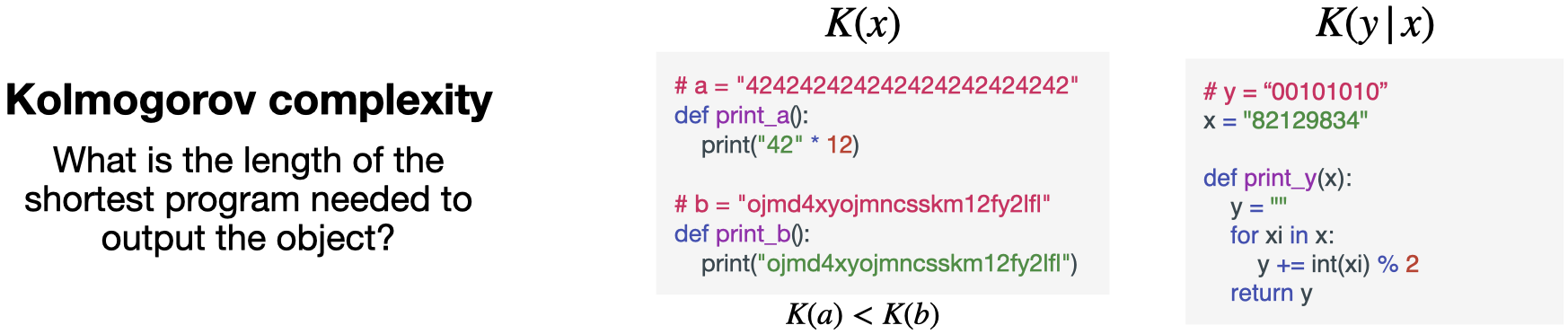
Kolmogorov complexity goes one step beyond Shannon information by dropping the assumption that the distribution $p$ is known to both the speaker and listener, and in fact drops the assumption that $x$ is drawn from any distribution at all. In Kolmogorov complexity, we instead only ask one thing: how compressible is $x$? The way that we do this is that we fix a Turing-complete programming language (Python, for instance), and we ask what is the length of the shortest program that I can write which outputs $x$. We denote this quantity $K(x)$.
Kolmogorov complexity
Given some finite string $x$ and a universal Turing machine $U$, the Kolmogorov complexity $K(x)$ is the length $l(r)$ (in bits) of the shortest binary program $r$ that prints $x$ and halts:
\[K(x) = \min_r \{l(r) : U(r) = x, r \in \{0, 1\}^* \}\]
Kolmogorov complexity has many intuitive properties that make it attractive as a measure of information quantity. The smaller and the more structure an object has — regularity, patterns, rules, etc. — the more easily it can be compressed using a short program and the lower its Kolmogorov complexity. For instance, a sequence with repeating patterns or a dataset that spans a low-dimensional subspace can be significantly compressed relative to its original size, and this results in low Kolmogorov complexity. In contrast, a random string devoid of any structure cannot be compressed at all and must in effect be “hard-coded”, making its Kolmogorov complexity equal to its original size in bits.
There’s also a conditional notion of Kolmogorov complexity that will be useful, denoted $K(y \mid x)$, which is equal to the length of the shortest program which takes $x$ as input and outputs $y$. Intuitively, this measures the amount of leftover information in $y$ given that we already know $x$. Conditional Kolmogorov complexity $K(y \mid x)$ is of course always less than or equal to $K(y)$ given that we have the option of simply ignoring the input $x$, and it can be significantly smaller than $K(y)$ when $x$ and $y$ share a lot of structure.
Sophistication and Occam’s razor
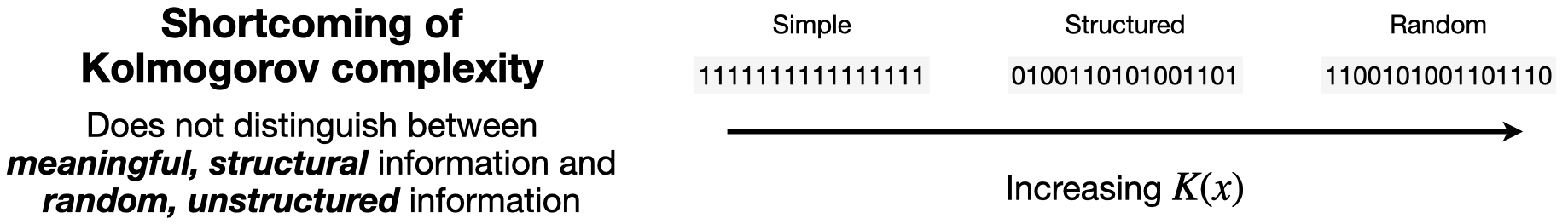
While powerful, Kolmogorov complexity isn’t completely satisfying as a universal measure of information quantity because it makes no distinction between meaningful, structural information and random, unstructured information. This is easiest to explain through examples. Consider a binary string $x$ that consists exclusively of a repeating sequence of $1$’s: it’s intuitively quite a simple object, and indeed $K(x)$ is quite low because we can print $x$ using a simple for-loop. Now, consider the opposite case of a binary string $y$ that consists of an entirely random sequence of $0$’s and $1$’s: $K(y)$ is maximally large because we have no other choice but to hard-code $y$. In one respect this makes sense — $y$ is incompressible, so in that respect it is indeed “complex”. But there is also a sense in which $y$ is strikingly simple, and in fact just as simple as a constant string like $x$. In particular, neither $y$ nor $x$ can really be said to have complex structure. They are equally boring. Even though $y$ must be described with a very large program, that program itself doesn’t contain much interesting logic outside of simply hard-coding bits, and the distribution from which $y$ might have been drawn would just take a few lines of code to define. In contrast, we can easily imagine a string $z$ that is also difficult to compress with high $K(z)$, but because it contains significant structure (i.e., interesting and sophisticated decompression code) rather than arbitrary randomness.
This distinction between structural and random information was important to Kolmogorov himself, who quantified it through a new metric called sophistication8. The idea is that we can consider strategies for compressing an object that work in two stages: first we encode some model of the object, and then second we encode the remaining bits of random information unaccounted for by the model. These compression strategies are called “two-part codes”. Let’s consider the model class of computable probability distributions as an example (although this also works with more general model classes). An optimal “two-part code” for an object $x$ that achieves the best possible compression is one that satisfies910:
\[K(x) = K(p_x) - \log_2 p_x(x)\]Here, $p_x$ is the probability distribution that we are using to model $x$ and $K(p_x)$ is the minimum number of bits that it takes to implement this probability distribution in a concrete computer program. Because $p_x$ might not be a perfect model of $x$, we also have to account for error correction bits, which in this case correspond to the ordinary Shannon information $-\log_2 p_x(x)$ (recall that Shannon information assumes access to the probability distribution from which $x$ is drawn, which we have accounted for in $K(p_x)$). There is always at least one model that satisfies this equality. For instance, $p_x$ can trivially put all its probability mass on $x$, in which case it takes $K(p_x) = K(x)$ bits to encode and achieves an error of $-\log_2p_x(x) = 0$ bits. However, in general, there can be many solutions. An interesting model to prefer above the others, though, is the one that is simplest:
\[p_x = \mathop{\arg\,\min}\limits_{p_x'} \{ K(p_x') : K(x) = K(p_x') - \log_2 p_x'(x) \}\]Note that in the above equation and for the rest of the blog post, the distribution $p_x$ does not just represent any model of $x$: it represents the simplest one that best compresses it. This particular model is not arbitrary, but rather is intrinsically defined purely in terms of $x$, which is why I have chosen to denote it $p_x$ where the subscript indicates the dependence on $x$.
Box: Distributions as models of individual objects?
By this point, for some readers a tension will have emerged. On the one hand, I’ve stated that Kolmogorov complexity is about individual objects and that $x$ represents an instance rather than a random variable. On the other hand, I’ve also been saying that we can use a probability distribution to model $x$, but probability distributions are generally models of… well, distributions and their random variables. So what gives? Is $x$ an individual object or is it a random variable drawn from a distribution?
We are indeed still talking about individual objects in this section, and we are making no assumptions whatsoever that $x$ has been drawn from a distribution. Nevertheless, for the purposes of compression, it can be convenient to pretend as if $x$ was drawn from a distribution. In particular, $x$ might look complex, but it might be possible to specify a simple distribution under which $x$ looks “typical” (i.e., it has high likelihood under this distribution, and is easily encoded through it). Admittedly, this can feel counter-intuitive — a distribution seems like a more complex thing than a single object that might have been drawn from that distribution — but it turns out to be true. A distribution is a generative process that can be simple, despite yielding objects of high complexity.
Here’s a simple example. Consider a long binary string $x$ consisting almost entirely of 1’s, but with a given percentage of 0’s peppered in. Directly encoding where each 0 occurs might be costly, but we can compress the string efficiently by specifying a binomial distribution with a particular success rate (a simple distribution that takes a few lines of code to implement) and then encoding $x$ under this distribution using $-\log_2p(x)$ bits. This does not mean that $x$ had to have actually come from a random binomially-distributed event; we are just pretending as if it had because $x$ looks typical under this distribution, and this can be leveraged for better compression. The distribution is simply a model.
I also want to close this discussion by emphasizing that even though $x$ is as single object, nothing stops us from considering a single object consisting of multiple draws from a distribution. Kolmogorov complexity is defined over strings, and we can easily represent something like an iid dataset by, for instance, concatenating individual datapoints together. In this case, the distribution that would best compress $x$ would likely chunk up the string and model it as a product of datapoint likelihoods. Computable probability distributions therefore form a flexible model class capable of compressing a wide variety of different objects.
There’s a nice parallel to machine learning theory here, and in particular the principle of Occam’s razor: we are looking for a simple model with low $K(p_x)$ that nevertheless accurately explains the data with low error $-\log_2 p_x(x)$. The complexity of this model $K(p_x)$ is what Kolmogorov described as the sophistication of the string $x$, and the Occam’s razor model $p_x$ is sometimes called the algorithmic minimal sufficient statistic910. Sophistication is precisely the quantity that we are looking for in order to distinguish between structured and unstructured information, where $K(x)$ alone was insufficient. If a string is too simple (e.g., a repeating pattern of $1’s$), it can be best compressed by a simple model with low $K(p_x)$. On the other hand, if a string is complex because of random noise rather than structure, $K(p_x)$ is still low because random noise distributions are easy to implement in just a few lines of code. It is only when a string has interesting and complex structure that $K(p_x)$ is high, meaning that the string is best compressed by a complex model.
I said earlier that sophistication is defined with respect to some class of models, and that computable probability distributions are just one option. For the rest of the post, to remain more general, I’ll therefore switch to the notation $m_x$ instead of $p_x$ to denote the Occam’s razor model of string $x$.
Defining compositionality through algorithmic information theory
We now have all the tools that we need to formally define compositional structure in data, and we can do so essentially just by replacing some of the language in our earlier definition with more precise mathematics. To briefly revisit this intuition, my central argument was that compositionality emerges from novel structure that is shared between an object’s parts. This is what that looks like in math:
Compositionality
An object $x$ is compositional with respect to some division into parts $x = [x_a, x_b]$ if:
\[K(m_x \mid m_{x_a}, m_{x_b}) > 0\]where the Occam’s razor model of the data $m_x = \mathop{\arg\,\min}\limits_{m_x’} \{ K(m_x’) : K(x) = K(m_x’) + l_{m_x}(x) \}$, and both $m_{x_a}$ and $m_{x_b}$ are defined similarly. The degree of compositional structure is $K(m_x \mid m_{x_a}, m_{x_b})$.
Note: $l_{m_x}(x)$ represents the unstructured information in $x$ left unspecified by the model $m_x$. For instance, for the model class of computable probability distributions $l_{m_x}(x) = -\log_2 m_x(x)$.
Once again, I need to emphasize that this definition only considers novel compositional structure in $x$ that wasn’t already present in $x_a$ or $x_b$ because it conditions on $m_{x_a}$ and $m_{x_b}$ — for instance, novel shared structure between two images, such as objects that appear in both but not in either individually. This definition does not preclude the possibility that the individual substrings $x_a$ and $x_b$ might themselves have compositional structure, and indeed this is an advantage. As I’ll show in section 3, this helps us easily think about hierarchical compositionality at different scales, since we can simply consider further divisions of the substrings $x_a$ and $x_b$ themselves.
Relation to other notions of compositionality and structure
I’ve argued for definition of compositionality based on novel algorithmic structural information. However, I don’t want to pretend that this is the only useful notion of compositionality out there — nor that it exists in a vacuum unrelated to existing notions. Rather, I want to argue that it provides a novel and general perspective that has unique implications for machine learning. Here, I’ll briefly highlight some connections to other frameworks for talking about compositionality, which will hopefully also serve to clarify properties of my definition.
Partial information decomposition
The most direct connection to existing theory is partial information decomposition (PID), an extension of Shannon information theory. PID attempts to decompose the information shared between a target $X$ and sources $X_a, X_b$ into unique, redundant, and synergistic components11. The synergistic term, denoted $\text{Syn}(X ; X_a, X_b)$, is the conceptual analog to my metric $K(m_x \mid m_{x_a}, m_{x_b})$: it is meant to quantify the information that arises solely from the interaction of the parts, rather than from any part in isolation12.
However, the move to algorithmic structural information provides unique advantages over PID. First, PID is fundamentally limited because the axioms of classical information theory become mutually incompatible when extended to this decomposition, meaning that no universally accepted definition for synergy exists13. This problem is absent in my framework: $K(m_x \mid m_{x_a}, m_{x_b})$ measures exactly the amount of novel structural information in $x$ that exists only due to synergistic interactions between $x_a$ and $x_b$, ignoring redundant and unique components, in a mathematically consistent way.
Second, PID struggles to quantify compositionality in the “part-whole” sense. If we define the target as simply the combination of the parts, $X = [X_a, X_b]$, standard synergy measures trivially vanish. As a result, applying PID to compositionality requires introducing external variables — such as distinguishing between a “word/sentence” and its “meaning” — to find any synergistic interaction1415. In contrast, $K(m_x \mid m_{x_a}, m_{x_b})$ naturally handles the emergence of structure when parts combine to form a whole, without needing to posit additional entities.
Finally, because Kolmogorov complexity can be seen as a generalization of Shannon information theory16, it retains the benefits of standard information theory while allowing us to model the internal structure of individual objects directly.
Complexity and sophistication
While building up to my final definition in this section, I’ve already contrasted it with both Kolmogorov complexity $K(x)$ and sophistication $K(m_x)$. However, it is still worth revisiting why we cannot simply use these existing measures — or simple derivatives of them — to quantify compositionality.
First, Kolmogorov complexity $K(x)$ itself is clearly insufficient. As we discussed, $K(x)$ is maximized for random strings, yet we intuitively know that white noise is not compositional. Conversely, if we tried to equate compositionality with compressibility (i.e., low $K(x)$), we would run into the opposite problem: a constant string of $0$’s would be deemed the “most compositional” object imaginable. Compositionality sits somewhere in the middle: it requires enough structure to be compressible, but enough complexity to be non-trivial.
Sophistication $K(m_x)$ gets us closer by focusing on the complexity of the structure (the model) rather than the noise. However, sophistication is agnostic to the kind of structure the object possesses. A model could be complex because it hard-codes a very long, flat, non-repeating rule, or it could be complex because it defines a rich, recursive hierarchy of reusable functions. Sophistication assigns a high value to both, failing to distinguish between “flat” complexity and the “deep” modular complexity we associate with compositionality. Recent variations of sophistication, such as Epiplexity17, ultimately suffer from the same limitation: they measure the amount of structure, not its architectural nature.
Perhaps the most compelling alternative candidate is the improvement in compression ratio that occurs when we join parts together. This idea, recently explored in the context of evolution and intelligence18, posits that structure exists when the whole is easier to explain than the sum of its parts: $K(x_a) + K(x_b) > K(x)$. This inequality captures the notion of redundancy or shared information. If $x_a$ and $x_b$ share structure, compressing them jointly in $x$ saves bits compared to compressing them separately. This is a necessary condition for compositionality — if parts don’t share structure, they can’t be composed — but it is not a sufficient one.
Consider the case where $x_a$ is a dataset of 1000 images, and $x_b$ is a 1001st image drawn from the exact same distribution. The combined dataset $x$ will satisfy $K(x_a) + K(x_b) > K(x)$ simply because we can reuse the existing model from $x_a$ to efficiently encode $x_b$. We have saved bits, but we haven’t learned anything new; we haven’t been forced to refactor our library or invent new concepts. We are just exploiting existing redundancy.
My definition, $K(m_x \mid m_{x_a}, m_{x_b}) > 0$, is strictly stronger. It requires not just that the whole be efficiently compressible, but that the model itself must change to achieve that compression. It can be shown that if $K(m_x \mid m_{x_a}, m_{x_b}) > 0$, then $K(x_a) + K(x_b) > K(x)$ necessarily follows, but the reverse is not true. By focusing on the novelty of the shared structure rather than just the presence of shared information, we distinguish between true compositionality (learning new rules) and mere statistical redundancy (applying old rules).
Grammars and functional programming
I would be remiss if I didn’t acknowledge that for many computer scientists and linguists, compositionality is already considered a “solved” problem. In the fields of programming language theory, formal semantics, and category theory, compositionality is traditionally defined by the Principle of Compositionality (often attributed to Frege or Montague). This principle states, roughly, that the meaning of a complex expression is determined by the meanings of its constituent parts and the rules used to combine them.
In this view, if we have a function $f$ (a rule) and parts $a, b$, the meaning of the whole is given by $M(f(a, b)) = F(M(a), M(b))$. This is the bedrock of functional programming and compiler design: we define a grammar or a type system a priori, and we say a program is compositional if it adheres to these structural rules. While these frameworks are incredibly powerful for designing artificial languages, they face significant limitations when trying to discover or quantify compositional structure in natural data.
The standard formalisms are prescriptive: they pre-specify a structure (a grammar, a logic, or a category) and ask whether the data fits. In contrast, the definition I’ve proposed is descriptive: it asks what structure is intrinsic to the data itself.Consider music. We all agree music is compositional; it reuses themes, rhythms, and harmonic progressions. But is there a formal grammar that perfectly describes all music that has ever been or will be written? Likely not. If we tried to force music into something like a Context-Free Grammar, we would inevitably fail to capture its nuance. However, using my definition, we don’t need to pre-define the rules of music. We simply ask: does the model $m_x$ that best compresses the symphony change and grow when we combine the movements $x_a$ and $x_b$? If the “whole” symphony forces us to invent (or discover) a new recurring motif or a key change that wasn’t justified by the parts in isolation, we have quantified its compositionality without ever writing down a formal grammar.
Another distinction lies in flexibility. In formal language theory, the “model” is usually a static set of production rules. In my framework, the model $m_x$ can be any computable program. It could be a symbolic grammar, yes, but it could also be a set of continuous weights in a neural network, a differential equation, or a program in a Turing-complete language. This is crucial because real-world data is often “soft” or noisy. A strict grammar says a sentence is either grammatical or it isn’t. An algorithmic information theory-based approach says a sentence is more or less compressible given a model. This allows us to apply the concept of compositionality to domains where clear boundaries don’t exist, such as images or sensor data, which resist formal symbolization.
Interestingly, there is a deep connection between my definition and the daily practice of functional programming: refactoring. In a sense, standard formalisms describe the end state of a perfectly factored program. My definition, $K(m_x \mid m_{x_a}, m_{x_b}) > 0$, quantifies the act of refactoring. When you realize that two disparate functions $x_a$ and $x_b$ share common logic, and you pull that logic out into a higher-order function in your library $m_x$, you have just satisfied the equation. You have created novel shared structure. In this way, my definition doesn’t replace the standard view; rather, it quantifies the emergence of the compositional structure that formal languages prize.
Section 3 — Implications and use-cases for AI
I hope that by this point my definition for compositionality is clear, at least at a high level. While the definition on its own may just be scientifically interesting to some readers, many more will surely be asking themselves: is it useful? I think the answer is yes, and that it might in fact have far reaching implications for AI. While I’m optimistic, these are still early days and I suggest readers take everything I’m about to say with a grain of salt. Testing these ideas empirically is very much a work in progress that I’ve only just begun to pursue.
Can compositionality be measured using this definition?
No, absolutely not. First, this formalism of compositionality is based on Kolmogorov complexity, which is well known to be uncomputable. Second, we need to infer the Occam’s razor model of some data, and no learning algorithm is that powerful.
But regardless of whether or not this definition of compositionality is computable, it can nevertheless prove useful at the conceptual level — after all, Kolmogorov complexity has stuck around since the 1960s despite being uncomputable because it helps us think about information in useful ways. One of the primary purposes of a definition is to unify diverse concepts and to simplify the language we use to talk about them, and I think this formalism of compositionality achieves that goal.
More importantly, $K(m_x \mid m_{x_a}, m_{x_b})$ can be estimated. Just as we can estimate Kolmogorov complexity using tractable compression algorithms, we can estimate compositionality as I’ve defined it here using compression and learning algorithms. In fact, in the context of modern machine learning, this might not even be overly challenging. Deep neural networks are powerful learners that, as a matter of empirical fact, have soft inductive biases to fit simple functions that compress their training data1920 — in other words, they already fit a good model $m_x$. What $K(m_x \mid m_{x_a}, m_{x_b})$ in turn quantifies is the degree to which a model changes as it sees more data, and there are already numerous methods for estimating this (or proxies of it) that broadly fit within the literature on “learning progress”21222317.
Beyond estimation, the definition also holds insights that might prove useful in the design of novel machine learning algorithms. As I’ll argue below, it provides a normative explanation for the success of depth in deep learning, and suggests that when we move towards non-iid data we should increase the depth of our models even further. Speaking of non-iid data, I’m particularly excited by the prospect of designing open-ended data curricula that are inspired by this definition, for which there are many paths forward. Crucially, the definition says that compositional models are perhaps straightforward to design, at least conceptually (we need only try to compress the data that we are given as well as possible), and that the emphasis should instead be on collecting compositional data on which to train these models. I think this is a big departure from most machine learning research on compositionality, which has often focused on more rigid architectural inductive biases.
Compositional structure all the way down
In real data, the underlying structure is almost always hierarchical.
On the scale of small image patches, there is already a substantial amount of compositional structure; the patch can be compressed using concepts such as edges and angles, for instance. Take a larger patch, and the repeating structures now correspond to simple shapes and textures which can themselves be compactly modeled on top of edge and angle features already present in the bank of concepts. In this way, even a single image can clearly be seen as a compositional object in which structures such as shapes and textures that frequently show up can be combined to form novel structures which are themselves reused. For instance, I’m currently sitting at my desk and I see rectangles everywhere: my laptop, the keys on the keyboard, my screen, my phone, my desk, my drawers — all of them are built up from rectangles. It thus makes sense to include the concept of a “rectangle” in a model that is meant to optimally compress my current field of view, and it makes sense to describe a rectangle on top of the concepts for edges and angles that do a good job of compressing data at smaller scales.
It’s fairly easy to describe what’s happening here using my definition of compositionality. When we consider two small patches of an image as $x_a$ and $x_b$, we get that for the joined patch $K(m_x \mid m_{x_a}, m_{x_b}) > 0$ because now it suddenly makes sense to include things like edges and angles in the model, since these types of things are shared between the two small patches. But when we consider joining two of those larger patches themselves, we can again detect novel compositional structure because the new model will benefit from describing things like simple textures and shapes which reoccur among the two larger patches.
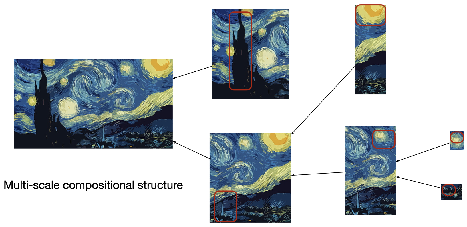
We can keep playing this game of joining larger segments of data to detect compositionality at increasingly large scales. In the compositionality literature, people typically only consider shared structure between individual datapoints (e.g., by modeling “objects” that get reused among images). I just showed how my definition can account for compositionality at smaller scales, such as within an individual image, but it can also account for compositionality at larger scales that consider sequences of observations in a non-stationary data stream. Over the course of a day, I spend much of my time at work and at home. The best compression strategy for a video feed of my life would involve constructing a model of each environment, which will be built off of the same sorts of objects (tables, chairs, etc.) that optimally compress data at the smaller scale. Similarly, optimal compression of longer scale visual events such as “a typical week in my life” will involve growing a model in a way that leverages existing concepts — my home, my workplace, and my frequent hobbies — in order to build larger ones that can themselves be reused to improve compression, such as my daily walk to and from work that itself happens again and again.
This all points to a significant advantage of my definition. In real, complex data that agents such as humans encounter, there is compositionality at all scales, both small and large. It is insufficient to think of compositionality at a single scale in isolation, such as scenes as being composed of objects, when the concepts at that scale are themselves built on top of smaller scale structures and contribute to the construction of larger scale ones. My definition makes it easy to talk about compositionality at all scales simultaneously using a single succinct equation, because it is agnostic to the size of the object being compressed and can be recursively applied to shorter and shorter segments of the object in a hierarchical fashion.
The success of deep learning
The core insight of deep learning is that complex data can be modeled through a cascade of hierarchically stacked functions which are themselves quite simple. Why does this work so well? If natural data is hierarchically compositional according to my definition — i.e., $K(m_x \mid m_{x_a}, m_{x_b}) > 0$ recursively — it suggests that in order to successfully model data at increasingly large scales we need to keep providing greater and greater capacity, with larger-scale models building on top of those at smaller scales. This is precisely what successive layers in a deep neural network do. We can interpret the features at a given layer as a “model” of the data at a particular scale; for instance, early layers in a CNN tend to represent local structure such as edges. The operation that gives us the features at the subsequent layer (e.g., convolution in a CNN) can then be thought of as capturing the novel structure $K(m_x \mid m_{x_a}, m_{x_b})$ that exists at a larger scale. Crucially, the functions performed at each layer do not have to be the same, which allows the network to continuously represent novel structure at larger scales in line with what we should expect from hierarchically compositional data.
While deep neural networks are ideally suited to representing hierarchical compositional structure in this way, the scale at which we use them is typically finite and predetermined. This is inevitable in the case of iid datasets, in which network features can at most represent structure that exists within a single datapoint, such as an image. Natural data that agents encounter is non-iid and, as I have argued, hierarchically compositional at all scales. This suggests a more radical sort of deep neural network architecture in which depth continues to grow, potentially unboundedly, in order to process data at increasingly large temporal scales; for instance, short video models building off of image model representations, longer video models building on top of those, and so on without any obvious stopping point so long as novel structure continues to be learned at these larger scales.
Data curricula and open-endedness
While machine learning often concerns itself with iid data, humans are generally confronted with data that extends deep in time and grows in complexity. This is of course quite natural — as we learn more and our internal model of the world grows, we’re driven by exploration to seek new data that we can’t yet explain. As a result, the stream of data collected by a human over the course of a lifetime is open-ended, and if we could stay in good health indefinitely it isn’t clear at what point our knowledge would saturate (at the very least, cultural knowledge seems to grow without limit).
In what way does an open-ended process produce data of ever-increasing complexity, or structure? Are we just talking about Kolmogorov complexity or sophistication? I don’t think so. It’s not just that knowledge grows arbitrarily in an open-ended process: it’s that it grows compositionally. Think of a school curriculum, for instance. We first learn about basic concepts — how to read, how to count, how to do arithmetic — and then we later build on top of these concepts to form new ones. Think of any complex domain or skill you know, and you can probably trace it back through a complex graph of knowledge you had previously gathered. Knowledge is rarely ever isolated; even in domains that we think of as very fact-based like history, we inevitably try to understand events in terms of how they relate to others.
What we have then is that a curriculum or an open-ended process must satisfy two properties. First, the new data that is collected in time must continually present novel structure that an agent can leverage to grow its model of the world. Second, there must be something about this novel structure that is shared with our prior knowledge so that we can build our world model in a hierarchical way that efficiently leverages past experience, and so that new experiences can shape our understanding of old ones.
By now it’s hopefully clear how my definition of compositionality can formalize these ideas. Consider a decomposition of some stream of data $x$ in which the final observation is $x_b$ and everything that came before it is $x_a$. Under what conditions will $K(m_x \mid m_{x_a}, m_{x_b}) > 0$? Clearly, if $x_b$ adds no novel structure, we’ll have that $m_x = m_{x_a}$ and $K(m_x \mid m_{x_a}, m_{x_b}) = 0$ as a consequence; the new observation did not change our model and we did not learn anything from it. $K(m_x \mid m_{x_a}, m_{x_b}) > 0$ therefore necessarily implies that learning has occurred and that the world model has changed. On the other hand, if $x_b$ is totally unrelated to what we previously knew, such that $x_b$ doesn’t help us better understand our past experience $x_a$ (and vice-versa), then we’ll have that $m_x = [m_{x_a}, m_{x_b}]$ and $K(m_x \mid m_{x_a}, m_{x_b}) = 0$ as well. This is what happens for instance when $x_b$ is a “pure fact” about the world that can’t be explained by building on top of prior knowledge, and must simply be memorized by brute force.
The two core properties of a curriculum — novel and shared structure — are therefore succinctly captured by my definition of compositionality. If the stream of data doesn’t grow knowledge, the model will remain the same and will fail to satisfy the definition. If the stream of data grows knowledge in a way that doesn’t leverage or refactor prior knowledge, it will also fail to satisfy the definition. Data streams that satisfy my definition necessarily entail a model that is continually growing into the future in a way where concepts grow on top of others and interact in complex networks. We can consider longer and longer streams, each time recursively asking whether or not my definition is still satisfied by the new observation, and if it is then we have an example of a truly open-ended process.
The implications here are quite obvious when we think of an agent that must not only model the data it has already seen, but also pick what data to see next – a problem all too relevant for modern AI. The solution I’m proposing here would be to use $K(m_x \mid m_{x_a}, m_{x_b})$ (or a proxy for it) as a reward signal for the agent’s policy that selects the next $x_b$. This is deeply related to the “learning progress” literature which tackles the problem of optimal exploration21, but it has the advantage that the agent’s world model will grow compositionally (as opposed to just growing a collection of independent facts). In my view, this research direction is the most promising application of my definition.
Box: Fractured/Entangled vs. Unified/Factored representations
As an aside, I recently read the fascinating paper “Questioning Representational Optimism in Deep Learning: The Fractured Entangled Representation Hypothesis” by Kumar et al.24, which found that neural representations which arise from open-ended curricula demonstrate significantly more compositional structure than those of models trained only on the final endpoints of these curricula (although they phrase things slightly differently, I think this is a fair interpretation of what they mean).
One conclusion the authors draw is that compression, while important, is not the only thing that a model should strive for — after all, the neural network they train on the final endpoint of a curriculum does a good job in terms of compression, but learns poor representations nonetheless. My theory of compositionality suggests a different conclusion, however: optimal compression is always what we should strive for when modeling, but crucially a curriculum might have significantly more compositional structure than its endpoint, and its optimal compression might therefore capture this compositional structure far better.
Take school curricula again, for instance. If my understanding of calculus builds off of prior concepts in algebra, I’ll be better able to jointly compress both through concept reuse. In contrast, if my only goal was to develop a compressed model of calculus in isolation, who knows what it would look like (imagine having learned calculus without knowing algebra first; I’m sure you would think of it in a very different way). There’s a crucial difference between compressing an entire curriculum versus compressing its endpoint alone. All of these interpretations of Kumar et al.’s fascinating findings are testable, and have important consequences for machine learning and the role of open-ended curricula.
Compositional structure diagrams
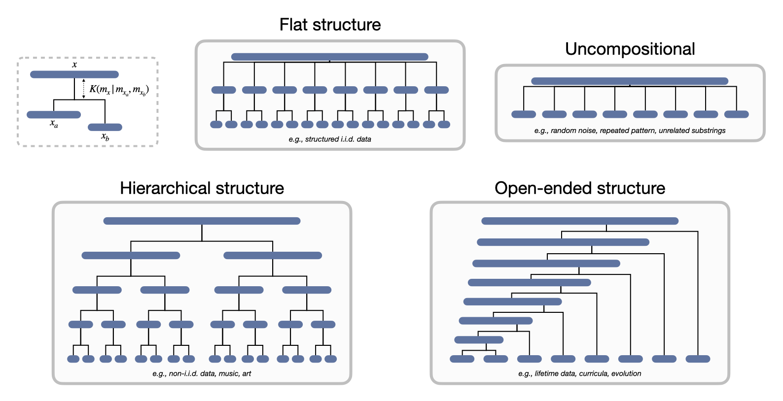
My intention with the above examples was to provide intuition for how my definition explains a breadth of different concepts spanning machine learning and cognitive science, but it’s important to emphasize that all of these examples are manifestations of the same underlying phenomenon. To better show how my definition provides a rich language for talking about diverse compositional structures, it can be helpful to map it onto a more visual medium, which I call a compositional structure diagram.
Essentially, a compositional structure diagram is a visual depiction of exactly what my definition says, compactly described in a tree. At the root we have the object $x$, which splits into two children $x_a$ and $x_b$, where we can then represent the novel compositional structure $K(m_x \mid m_{x_a}, m_{x_b})$ by the height of the branch that merges the two children. We can also do this for the children $x_a$ and $x_b$ themselves, and continue recursively until at the leaves we’re left with indivisible parts (e.g., single bits). Note that we can consider different hierarchical decompositions of the same object by picking different splits at each node, but some might make more sense to look at then others; for instance, decompositions that lead to deeper trees or decompositions with “maximal” trees that have the larger summed $K(m_x \mid m_{x_a}, m_{x_b})$ (see below for a longer discussion around this point).
In Figure 8, I’ve shown what the compositional structure diagram might look like for several kinds of objects that I’ve discussed above. At a glance, this gives us an intuitive sense of the object’s intrinsic compositional structure, and it shows us where in the object and at which scales that compositional structure emerges. It shows us how larger structures are built off of novel structure shared at smaller scales, like how concepts build off of others, and it shows us how this happens recursively through the object. There’s a nice analogy to be made to phylogenetic trees in biology, but whereas phylogenetic trees show a plausible story of how genetic structure diverges over time and splits off into new species, compositional structure diagrams show a plausible story of how structures merge to form novel ones (which, according to a recent theory of evolution called symbiogenesis18, might actually be how we should think of phylogenetic histories in the first place).
What decompositions should we consider?
The definition of compositionality I’ve proposed here clearly depends on how we decompose a string into substrings: $K(m_x \mid m_{x_a}, m_{x_b})$ depends on our choice for $x_a$ and $x_b$, and different choices will give different answers. These choices are compounded when we want to consider recursive tree-based decompositions like the ones I highlighted above. What should we make of this? Is there a “correct” decomposition that makes more sense to consider than others? If not, then how should we think about these different decompositions and the results they give? Are they giving us different, but potentially complementary views on the compositional structure of an object?
The first thing to say at the outset here is that I don’t know the answers for certain, and that everything from this point on in this section is largely conjecture based on intuition. I should also note that if your head is starting to hurt, this is a good section to skip as it is fairly technical.
On the one hand, it’s conceivable that the interesting decompositions we should consider might depend on the kind of data we’re dealing with. For instance, with iid data, the ordering of datapoints is irrelevant: we’re really dealing with a set of strings rather than one large string. Perhaps, then, we should just consider the amount of novel structure added when we join subsets of increasingly large sizes, for instance the quantities $C_n(D) = \mathbb{E} [ K(m_{[x_1, …, x_n]} \mid m_{x_1}, …, m_{x_n}) ]$ for $n=1..len(D)$, where $(x_1, …, x_n) \sim D$ so that we’re sampling $n$ datapoints uniformly from an iid dataset $D$. If we’re instead dealing with non-iid data that is nevertheless stationary in time, perhaps it makes more sense to consider a balanced binary tree as the hierarchical decomposition where we merge pairs of datapoints, and then pairs of pairs, and so on, since such a decomposition would be time-invariant. If we’re dealing with nonstationary streaming data, like a curriculum constructed by an intelligent agent, the most interesting decomposition might be one in which we keep joining each new datapoint to the entire history seen thus far.
On the other hand, I have the intuition that the most interesting recursive decomposition to consider in general is the one that leads to maximal trees. What I mean by a maximal tree here is that when we sum the $K(m_x \mid m_{x_a}, m_{x_b})$ terms at each node in the decomposition, we get a larger value than for any other possible recursive decomposition of $x$. We can call this maximal tree $T_{max}(x)$ and its corresponding sum $C_{T_{max}}(x)$. There are many reasons why this decomposition is interesting and convenient for talking about compositionality.
First, the maximal tree will always join objects that share novel structure and parts, which maps on to how we intuitively think about compositionality. In contrast, if we were looking at minimal trees, we would be joining objects that are either structurally identical or algorithmically independent.
Second, while $C_{T_{max}}(x)$ is lower-bounded by $K(m_x)$ (it is a possible strategy for compressing the final model), there are strings for which $C_{T_{max}}(x) > K(m_x)$. This means that the quantity $C_{T_{max}}(x)$ doesn’t simply reduce to sophistication but rather quantifies something else. Of course, for this to be true we actually have to make sure that $C_{T_{max}}(x) > K(m_x)$ in strings we intuitively consider compositional, and conversely that $C_{T_{max}}(x) = K(m_x)$ in strings we believe are uncompositional. While I have yet to show either of these things theoretically or empirically, I think that they will hold. In any case, what I do know is that this is not the case if we consider minimal trees: for minimal trees, there is always a trivial solution that merges every individual bit of a string in one single merge, meaning that for all $x$, $C_{T_{min}}(x) = K(m_x)$.
Third, we should hope that if a string is measured to be “compositional” by some metric, it remains compositional when it is embedded as a substring within a larger structure. If this were not the case, it would mean that the compositionality of an object is context-dependent, and we wouldn’t be able to say that compositionality is an intrinsic and objective property of the object. $C_{T_{max}}(x)$ happens to have this property, so we can say that it is a recursively-consistent metric. In particular, if a substring appears in its superstring’s maximal tree, then the substring’s maximal tree is also guaranteed to be a subtree in the superstring’s maximal tree (this sentence may take several reads to digest, apologies).
Fourth, considering the maximal tree solves an annoying technical problem: why only consider binary joining operations? Why not join triplets, or quadruplets of substrings? While this choice may seem arbitrary, it is cleanly resolved if we only consider maximal trees. The reason is that the novel structure generated from joining a triplet is guaranteed to be less than or equal to what is generated from a pair of binary joining operations, where we first join two of the substrings, and then join the result with the remaining substring. This is easy to prove on paper, and the proof extends by induction to quadruplets and so on. Once again, minimal trees give the opposite result because they always admit a trivial solution that merges every individual bit in one shot.
Hopefully I’ve made a convincing argument for why maximal tree decompositions are particularly interesting, and might get at the heart of an object’s intrinsic compositional structure. Once again though, a lot of theoretical and empirical work still needs to be done to back up these claims, and my reasoning may very well be flawed.
Conclusion
My work on formally defining compositionality did not start out of nowhere: it arose for a particular reason. I had recently started my PhD and was interested in designing models that can flexibly generalize like humans do when we think, dynamically composing concepts in order to adapt to novel situations. The further I got into my projects, however, the more I felt like I no longer understood the original goal, unable to explain what the scientific problems were or why the approaches I was pursuing would work. Eventually, I started to realize that we take compositionality for granted, using it in our vocabulary for talking about AI without having any real clue as to what it means.
This work has filled that conceptual gap for me, and given me renewed clarity on my research and scientific interests. I hope that it can serve a similar purpose for others in the field who are reading this blog post and interested in compositionality. However, like all scientific formalisms, I think that the real significance of these ideas is in the serendipitous directions they may lead future research. For me, having a new way to think and talk about compositionality more precisely has opened the flood gates: I see new research ideas, applications, and connections to other fields everywhere I look. I’ve tried to highlight some of these here, but my biggest hope in writing this blog post is that it has a similar stimulating effect for others, and that research into compositionality benefits from a new pool of creative ideas.
To cite this blog post, please use the following:
@online{elmoznino2025definingcompositionalstructure
    author = {Eric Elmoznino},
    title = {Defining and quantifying compositional structure},
    year = {2025},
    url = {https://ericelmoznino.github.io/blog/2025/08/18/defining-compositionality/},
}
Acknowledgements
A special thanks to Tejas Kasetty, who was instrumental in helping me develop this theory of compositionality from the ground up. I’m also grateful to my supervisors Guillaume Lajoie, Yoshua Bengio, and (unofficially) Dhanya Sridhar, as well as to my fellow graduate students Tom Marty, Léo Gagnon, Sarthak Mittal, and David Dobre, all of whom provided crucial feedback that helped me greatly improve this blog post.
References
-
Fukushima, K. (1980). Neocognitron: A self-organizing neural network model for a mechanism of pattern recognition unaffected by shift in position. Biological cybernetics, 36(4), 193-202. ↩
-
Bronstein, M. M., Bruna, J., Cohen, T., & Veličković, P. (2021). Geometric Deep Learning: Grids, Groups, Graphs, Geodesics, and Gauges (No. arXiv:2104.13478). arXiv. https://doi.org/10.48550/arXiv.2104.13478 ↩
-
Stanley, K. O. (2007). Compositional pattern producing networks: A novel abstraction of development. Genetic programming and evolvable machines, 8(2), 131-162. ↩
-
Mildenhall, B., Srinivasan, P. P., Tancik, M., Barron, J. T., Ramamoorthi, R., & Ng, R. (2021). Nerf: Representing scenes as neural radiance fields for view synthesis. Communications of the ACM, 65(1), 99-106. ↩
-
Ballé, J., Versari, L., Dupont, E., Kim, H., & Bauer, M. (2024). Good, Cheap, and Fast: Overfitted Image Compression with Wasserstein Distortion (No. arXiv:2412.00505). arXiv. https://doi.org/10.48550/arXiv.2412.00505 ↩
-
Liao, I., & Gu, A. (2025). ARC-AGI Without Pretraining. Retrieved from https://iliao2345.github.io/blog_posts/arc_agi_without_pretraining/arc_agi_without_pretraining.html ↩
-
Kolmogorov, A. (1965). Three approaches to the quantitative definition of information. Problems of Information Transmission, 1(1), 1–7. ↩
-
Kolmogorov, A. (1973). Talk in information theory symposium. Tallinn, Estonia. ↩
-
Grunwald, P. D., & Vitanyi, P. M. B. (2008). Algorithmic information theory (No. arXiv:0809.2754). arXiv. https://doi.org/10.48550/arXiv.0809.2754 ↩ ↩2
-
Vitanyi, P. (2006). Meaningful Information (No. arXiv:cs/0111053). arXiv. https://doi.org/10.48550/arXiv.cs/0111053 ↩ ↩2
-
Williams, P. L., & Beer, R. D. (2010). Nonnegative decomposition of multivariate information (No. arXiv:1004.2515). arXiv. https://doi.org/10.48550/arXiv.1004.2515 ↩
-
Tax, T. M., Mediano, P. A., & Shanahan, M. (2017). The partial information decomposition of generative neural network models. Entropy, 19(9), 474. ↩
-
Hendrik Matthias, P., Makkeh, A., Wibral, M., & Gutknecht, A. J. (2025). Novel Inconsistency Results for Partial Information Decomposition (No. arXiv:2512.16662). arXiv. https://arxiv.org/abs/2512.16662 ↩
-
Socolof, M., Vigly, J. H., Futrell, R., Sordoni, A., & O’Donnell, T. (2022). Measuring morphological fusion using partial information decomposition. In Proceedings of the 29th International Conference on Computational Linguistics (pp. 44-54). ↩
-
Socolof, M., Cheung, J. C. K., Wagner, M., & O’Donnell, T. (2022). Characterizing idioms: Conventionality and contingency. In Proceedings of the 60th Annual Meeting of the Association for Computational Linguistics (Volume 1: Long Papers) (pp. 4024-4037). ↩
-
Grünwald, P. D., & Vitányi, P. M. (2003). Kolmogorov complexity and information theory. With an interpretation in terms of questions and answers. Journal of Logic, Language and Information, 12(4), 497-529. ↩
-
Finzi, M., Qiu, S., Jiang, Y., Izmailov, P., Kolter, J. Z., & Wilson, A. G. (2026). From Entropy to Epiplexity: Rethinking Information for Computationally Bounded Intelligence (arXiv:2601.03220). arXiv. https://doi.org/10.48550/arXiv.2601.03220 ↩ ↩2
-
Agüera y Arcas, B. (2025). What Is Intelligence?: Lessons from AI About Evolution, Computing, and Minds. Cambridge, MA: MIT Press. ↩ ↩2
-
Wilson, A. G. (2025). Deep Learning is Not So Mysterious or Different (arXiv:2503.02113). arXiv. https://doi.org/10.48550/arXiv.2503.02113 ↩
-
Goldblum, M., Finzi, M., Rowan, K., & Wilson, A. G. (2023). The No Free Lunch Theorem, Kolmogorov Complexity, and the Role of Inductive Biases in Machine Learning (arXiv:2304.05366). arXiv. https://doi.org/10.48550/arXiv.2304.05366 ↩
-
Schmidhuber, J. (2010). Formal Theory of Creativity, Fun, and Intrinsic Motivation (1990–2010). IEEE Transactions on Autonomous Mental Development, 2(3), 230–247. IEEE Transactions on Autonomous Mental Development. https://doi.org/10.1109/TAMD.2010.2056368 ↩ ↩2
-
Linke, C., Ady, N. M., White, M., Degris, T., & White, A. (2020). Adapting Behavior via Intrinsic Reward: A Survey and Empirical Study. Journal of Artificial Intelligence Research, 69, 1287–1332. https://doi.org/10.1613/jair.1.12087 ↩
-
Zhang, X., Li, X., Dou, D., & Wu, J. (2020). Measuring Information Transfer in Neural Networks (arXiv:2009.07624). arXiv. https://doi.org/10.48550/arXiv.2009.07624 ↩
-
Kumar, A., Clune, J., Lehman, J., & Stanley, K. O. (2025). Questioning Representational Optimism in Deep Learning: The Fractured Entangled Representation Hypothesis (No. arXiv:2505.11581). arXiv. https://doi.org/10.48550/arXiv.2505.11581 ↩